Algebra 2 - Part 3: Function Transformations, Equations, Trigonometry, and Modeling

December 27, 2025

Function Transformations

Function transformation is the process of changing the graph of a function by shifting, stretching, compressing, or reflecting it to create a new, related function.

Shifting Functions

\[\Large g(x) = f(x - a) + b\]

From the video above, you can see that the formula is \(f(x) = (x - a)^2 + b\). When we changed the value of \(a\), it shifted to the right (when \(a \gt 0\)) or to the left (when \(a \lt 0\)). When we changed the value of \(b\), it is shifted up (when \(b \gt 0\)) or down (when \(b \lt 0\)).

Let's find a formula for shifting functions. Here is an example.

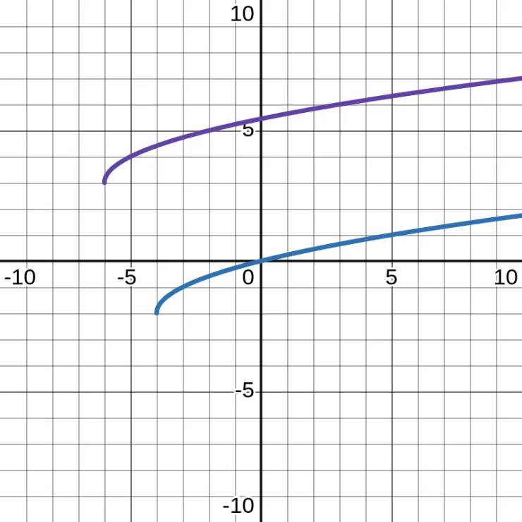
Given that \(f(x) = \sqrt{x + 4} - 2\), write an expression for \(g(x)\) in terms of \(x\).

\begin{aligned} g(x) &= f(x - a) + b \\\\ &= f(x - (-2)) + 5 \\\\ &= f(x + 2) + 5 \\\\ &= \sqrt{x + 2 + 4} - 2 + 5 \\\\ &= \sqrt{x + 6} + 3 \end{aligned}

Reflecting Functions

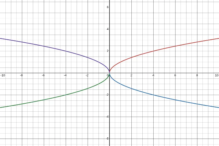
Here is an example of Reflecting Functions. We have 4 lines on the graph above.

The red line, \(a(x) = \sqrt{x}\). This is the standard square-root curve, starting at \(x = 0\) and increasing to the right.
The blue line, \(b(x) = -a(x)\). Multiplying by \(-1\) reflects the red line across the x-axis. Every positive output becomes negative.
The green line, \(c(x) = b(-x)\). Replacing \(x\) with \(-x\) reflects the blue graph across the y-axis. This flips the graph horizontally.
The purple line, \(d(x) = -c(x)\). Multiplying the green graph by \(-1\) reflects it across the x-axis again.

Symmetry of Functions

More generally, symmetry of functions refers to how a graph behaves under reflection. An even function has y-axis symmetry and satisfies \(f(x)=f(-x)\). An odd function has origin symmetry and satisfies \(f(x)=-f(-x)\).

Even Functions

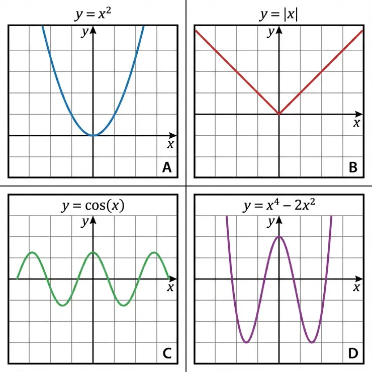
Odd Functions

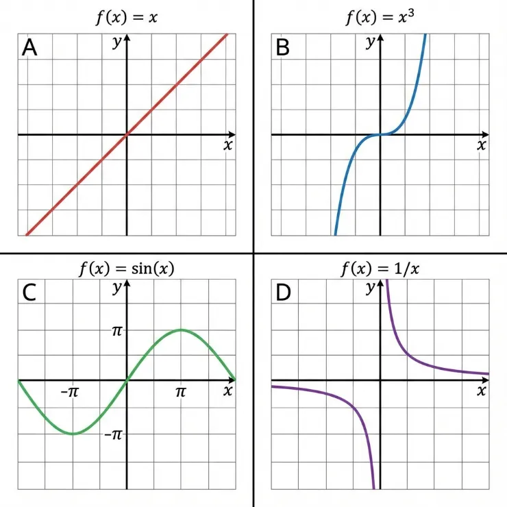
Symmetry of Monomials

Based on the previous explanation in Symmetry of Functions, we can conclude that:

Even is \(f(x)=f(-x)\).
Odd is \(f(x)=-f(-x)\).
Otherwise, it is neither even nor odd.

Let's examine those equations or rules with some examples.

\begin{aligned} g(x) &= 3x^{2} \\\\ g(-x) &= 3(-x)^{2} \\\\ &= 3(x^{2}) \\\\ &= 3x^{2} \\\\ &= g(x) \end{aligned}
\begin{aligned} h(x) &= -2x^{5} \\\\ h(-x) &= -2(-x)^{5} \\\\ &= -2(-x^{5}) \\\\ &= 2x^{5} \\\\ &= -h(x) \end{aligned}

From those examples, we can conclude that in monomials if the degree (\(n\)) is even, then the function (\(f\)) is even; if the degree is odd, then the function is odd.

\[\Large f(x) = ax^n\]

Scaling Functions

Scaling functions involves stretching or compressing their graphs either vertically (affecting y-values) by multiplying the whole function (\(c\cdot f(x)\)) or horizontally (affecting x-values) by replacing \(x\) with \(kx\), changing the steepness/width and intercepts.

Vertical Scaling

\[\Large g(x) = c \cdot f(x)\]

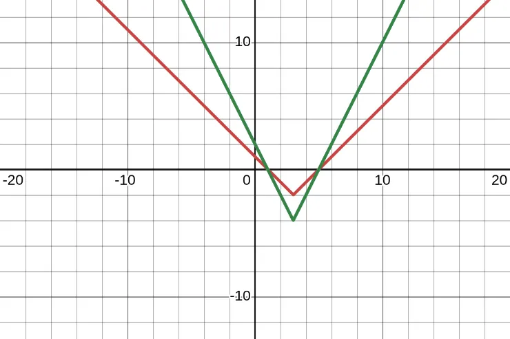
Here is an example. The graph of the function \(f(x) = |x - 3| - 2\). What is the graph of \(g(x) = 2|x - 3| -4\)?

Here is the answer in the table format.

\(x\)	\(f(x)\)	\(h(x)\)
0	1	2
3	-2	-4
5	0	0

Here is the answer in the graph format.

Horizontal Scaling

\[\Large g(x) = f(kx)\]

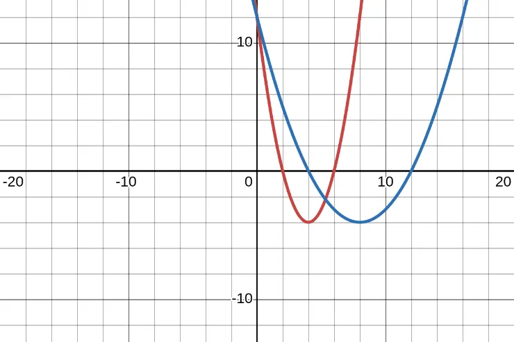
Here is an example. The graph of the function \(f(x) = (x - 4)^2 - 4\). What is the graph of \(g(x) = (\frac{x}{2} - 4)^{2} - 4\)?

Here is the answer in the table format.

\(x\)	\(\frac{1}{2}x\)	\(g(x) = f(\frac{1}{2}x)\)
4	2	\(g(4) = f(2) = 0\)
8	4	\(g(8) = f(4) = -4\)
12	6	\(g(12) = f(6) = 0\)

Here is the answer in the graph format.

Equations

Equations are mathematical statements showing two expressions are equal, linked by an equals sign (=). They express relationships between numbers and variables (unknowns), and solving them means finding variable values that make the statement true.

Rational Equations

Equations with rational expressions (rational equations) involve variables in the numerator or denominator, solved by finding the Least Common Denominator (LCD) to clear fractions, then solving the resulting polynomial equation, always remembering to check for extraneous solutions (values making the original denominator zero). Key steps include factoring denominators, finding the LCD, multiplying all terms by the LCD to eliminate fractions, solving the simpler equation, and verifying solutions against the original equation's domain restrictions (e.g., \(x\ne 0,x\ne 2\)).

Here are examples.

\begin{aligned} \frac{x^{2}-10x+21}{3x-12} &= \frac{x-5}{x-4} \\\\ \frac{x^{2}-10x+21}{3(x-4)} &= \frac{x-5}{x-4} \\\\ \frac{x^{2}-10x+21}{3} &= x-5 \\\\ x^{2}-10x+21 &= 3x-15 \\\\ x^{2}-13x+36 &= 0 \\\\ (x-4)(x-9) &= 0 \\\\ x-4=0 &\text{ or } x-9=0 \\\\ x=4 &\text{ or } x=9 \end{aligned}
\begin{aligned} \frac{-2x+4}{x-1} &= \frac{3}{x+1}-1 \\\\ (x+1)(x-1)\frac{-2x+4}{x-1} &= (\frac{3}{x+1}-1)(x-1)(x+1) \\\\ (x+1)(-2x+4) &= 3x-3-1(x-1)(x+1) \\\\ (x+1)(-2x+4) &= 3x-3-(x^{2}-1) \\\\ -2x^{2}+4x-2x+4 &= 3x-3-x^{2}+1 \\\\ -2x^{2}+2x+4 &= -x^{2}+3x-2 \\\\ -x^{2}-x+6 &= 0 \\\\ x^{2}+x-6 &= 0 \\\\ (x+3)(x-2) &= 0 \\\\ x+3=0 &\text{ or } x-2=0 \\\\ x=-3 &\text{ or } x=2 \end{aligned}

Finding Inverses of Rational Functions

To find the inverse of a rational function, replace \(f(x)\) with \(y\), swap \(x\) and \(y\), then solve the new equation for \(y\) by clearing denominators and isolating \(y\), finally replacing \(y\) with \(f^{-1}(x)\) and noting domain restrictions. Here is an example.

\begin{aligned} f(x) &= \frac{2x+5}{4-3x} \\\\ y &= \frac{2x+5}{4-3x} \\\\ x &= \frac{2y+5}{4-3y} \\\\ 4x-3yx &= 2y+5 \\\\ -3yx-2y &= 5-4x \\\\ y(-3x-2) &= 5-4x \\\\ y &= \frac{5-4x}{-3x-2} \\\\ f^{-1}(x) &= -1 \cdot \frac{5-4x}{-3x-2} \\\\ &= \frac{4x-5}{3x+2} \end{aligned}

Square-root Equations & Extraneous Solutions

Square root equations involve a variable under a radical sign (\(\sqrt{}\)), solved by isolating the radical, then squaring both sides to eliminate the root, which often results in a linear or quadratic equation to solve. The crucial step is to check solutions in the original equation, as squaring can introduce extraneous (false) solutions that don't work.

An extraneous solution is a potential answer to a math equation that appears valid during the solving process but fails to work when plugged back into the original equation.

Here is an example.

\begin{aligned} \sqrt{x} &= 2x - 6 \\\\ (\sqrt{x})^{2} &= (2x - 6)^{2} \\\\ x &= 4x^{2} - 24x + 36 \\\\ 0 &= 4x^{2} - 25x + 36 \\\\ x &= \frac{-1 \cdot -25 \pm \sqrt{(-25)^{2} - 4 \cdot 4 \cdot 36}}{2 \cdot 4} \\\\ x &= \frac{25 \pm \sqrt{49}}{8} \\\\ x &= \frac{25 \pm 7}{8} \\\\ x = \frac{32}{8} = 4 &\text{ or } x = \frac{18}{8} = 2\frac{2}{8} = 2.25 \\\\ \sqrt{4} = 2(4) - 6 &\qquad \sqrt{2.25} = 2(2.25) - 6 \\\\ 2 = 8 - 6 &\qquad 1.5 = 4.5 - 6 \\\\ 2 = 2 &\qquad 1.5 \neq -1.5 \end{aligned}

From the example above, we can see that 2.25 is an extraneous solution.

We used the Quadratic Formula, which we learned in Algebra (Part 3), to solve the equation. This gives two candidate solutions. Each candidate must be checked in the original equation, because some solutions may be extraneous. If all candidates are extraneous, then the equation has no solution.

Cube-root Equations

A cube root equation involves finding a number that, when multiplied by itself three times, equals a given number, represented as \(\sqrt[3]{x}=a\) or \(x^{1/3}=a\). Let's solve a cube-root equation. Here is an example.

\begin{aligned} -\sqrt[3]{y} &= 4\sqrt[3]{y} + 5 \\\\ -5\sqrt[3]{y} &= 5 \\\\ \sqrt[3]{y} &= -1 \\\\ (\sqrt[3]{y})^{3} &= (-1)^{3} \\\\ y &= -1 \end{aligned}

Quadratic Systems

A quadratic system involves equations with variables raised to the second power, most commonly a linear-quadratic system (line + parabola) or a quadratic-quadratic system (two curves like parabolas/circles), solved by finding (x, y) points satisfying all equations. Here are examples.

A Line and a Parabola

The parabola given by \(y = 3x^{2} - 6x + 1\) and the line given by \(y - x + 1 = 0\) are graphed.

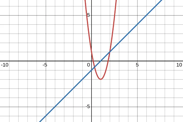
One intersection point that is clearly identifiable from the graph is (2, 1).

Find the other intersection point!

\begin{aligned} y &= 3x^{2} - 6x + 1 \\\\ y - x + 1 &= 0 \\\\ y &= x - 1 \\\\ x - 1 &= 3x^{2} - 6x + 1 \\\\ 0 &= 3x^{2} - 7x + 2 \\\\ &= 3x^{2} - 6x - x + 2 \\\\ &= 3x(x - 2) -1(x - 2) \\\\ &= (x - 2)(3x - 1) \\\\ x - 2 = 0 &\text{ or } 3x - 1 = 0 \\\\ x = 2 &\text{ or } x = \frac{1}{3} \end{aligned}

We already knew that if \(x = 2\), then \(y = 1\). Let's find \(y\) if \(x = \frac{1}{3}\).

\begin{aligned} y &= x - 1 \\\\ &= \frac{1}{3} - 1 \\\\ &= -\frac{2}{3} \end{aligned}

So, the other intersection point is (\(\frac{1}{3}\), \(-\frac{2}{3}\)).

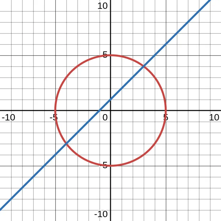
A Line and a Circle

What are the solutions to the system of equations \(y = x + 1\) and \(x^{2} + y^{2} = 25\)?

\begin{aligned} x^{2} + y^{2} &= 25 \\\\ x^{2} + (x + 1)^{2} &= 25 \\\\ x^{2} + x^{2} + 2x + 1 &= 25 \\\\ 2x^{2} + 2x + 1 &= 25 \\\\ 2x^{2} + 2x - 24 &= 0 \\\\ x^{2} + x - 12 &= 0 \\\\ (x + 4)(x - 3) &= 0 \\\\ x = -4 &\text{ or } x = 3 \end{aligned}

We already have \(x\) now. Let's find \(y\)!

If \(x = -4\), then \(y = -4 + 1 = -3\).
If \(x = 3\), then \(y = 3 + 1 = 4\).

So, the solutions are (-4, -3) and (3, 4).

Trigonometry

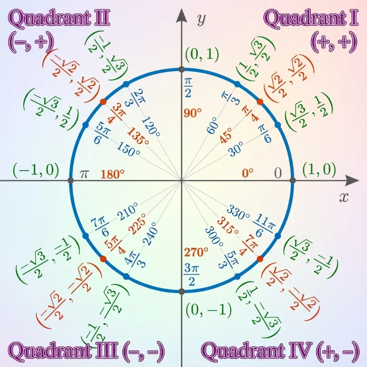
Unit Circle

The unit circle is a circle with a radius of 1, centered at the origin (0,0) on a coordinate plane, fundamentally used in trigonometry to define sine, cosine, and tangent for any angle. For any point \((x,y)\) on the circle, \(x=\cos (\theta )\) and \(y=\sin (\theta )\), with the angle \(\theta \) measured from the positive x-axis.

\[\Large \tan \theta = \frac{\sin \theta}{\cos \theta}\]

In trigonometry, the sides of a right triangle are named based on their position relative to a chosen angle. These names—hypotenuse, opposite, and adjacent—help us define and understand trigonometric ratios such as sine, cosine, and tangent.

Hypotenuse: the longest side of a right triangle, opposite the right angle.
Opposite side: the side directly across from the angle θ.
Adjacent side: the side next to the angle θ that is not the hypotenuse.

\[ \sin\theta = \frac{\text{opposite}}{\text{hypotenuse}}, \quad \cos\theta = \frac{\text{adjacent}}{\text{hypotenuse}}, \quad \tan\theta = \frac{\text{opposite}}{\text{adjacent}} \]

Here are examples. You can verify these by using a calculator.

\(\sin(50^\circ)=0.77\)
\(\cos(100^\circ)=-0.17\)
\(\tan(120^\circ)=-1.73\)

Radians

A radian is a unit for measuring angles, defined as the angle created when an arc length on a circle equals the circle's radius, making it a natural unit in math and science, where a full circle is \(2\pi \) radians (about \(360^{\circ }\)) and a half circle is \(\pi \) radians (\(180^{\circ }\)).

Here are rules of conversion:

Degrees to Radians: Multiply by \(\frac{\pi }{180}\).
Radians to Degrees: Multiply by \(\frac{180}{\pi }\).

Here are examples of converting degrees to radians and vice versa.

\(150^\circ \cdot \frac{\pi}{180} = \frac{150\pi}{180} = \frac{5\pi}{6} \text{radians}\)
\(\frac{-\pi}{3}\text{radians} \cdot \frac{180}{\pi} = \frac{-180}{3} = -60^\circ\)

Quadrants

Radian angles determine quadrants on a unit circle, where Quadrant I (0 to \(\frac{\pi }{2}\)) (+, +), Quadrant II (\(\frac{\pi }{2}\) to \(\pi \)) (-, +), Quadrant III (\(\pi \) to \(\frac{3\pi }{2}\)) (-, -), and Quadrant IV (\(\frac{3\pi }{2}\) to \(2\pi \)) (+, -) represent divisions of the circle, with \(2\pi \) completing a full revolution.

Pythagorean Trigonometric Identity

\[\Large x^{2} + y^{2} = 1\]

The Pythagorean identity tells us that no matter what the value of \(\theta\) is, \(\sin^{2}\theta+\cos^{2}\theta\) is equal to 1. Here are examples.

\(\theta_1\) is located in Quadrant III, and \(\cos(\theta_1) = -\frac{3}{5}\). \(\sin(\theta_1)\) = ?

\begin{aligned} \sin^{2}(\theta_1) + \cos^{2}(\theta_1) &= 1 \\\\ \sin^{2}(\theta_1) + (-\frac{3}{5})^{2} &= 1 \\\\ \sin^{2}(\theta_1) &= 1 - (-\frac{3}{5})^{2} \\\\ \sin^{2}(\theta_1) &= 1 - \frac{9}{25} \\\\ \sin^{2}(\theta_1) &= \frac{16}{25} \\\\ \sqrt{\sin^{2}(\theta_1)} &= \sqrt{\frac{16}{25}} \\\\ \sin(\theta_1) &= \pm\frac{4}{5} \end{aligned}

Because \(\sin(\theta_1)\) is located in Quadrant III, so its sine value must be negative, \(\sin(\theta_1) = -\frac{4}{5}\).
\(\theta_1\) is located in Quadrant II, and \(\sin(\theta_1) = -\frac{9}{41}\). \(\cos(\theta_1)\) = ?

\begin{aligned} \sin^{2}(\theta_1) + \cos^{2}(\theta_1) &= 1 \\\\ (\frac{9}{41})^{2} + \cos^{2}(\theta_1) &= 1 \\\\ \cos^{2}(\theta_1) &= 1 - (\frac{9}{41})^{2} \\\\ \cos^{2}(\theta_1) &= 1 - \frac{81}{1681} \\\\ \cos^{2}(\theta_1) &= \frac{1600}{1681} \\\\ \sqrt{\cos^{2}(\theta_1)} &= \sqrt{\frac{1600}{1681}} \\\\ \cos(\theta_1) &= \pm\frac{40}{41} \end{aligned}

Because \(\cos(\theta_1)\) is located in Quadrant II, so its cosine value must be negative, \(\cos(\theta_1) = -\frac{40}{41}\).

Graph of \(sin(x)\), \(cos(x)\), and \(tan(x)\)

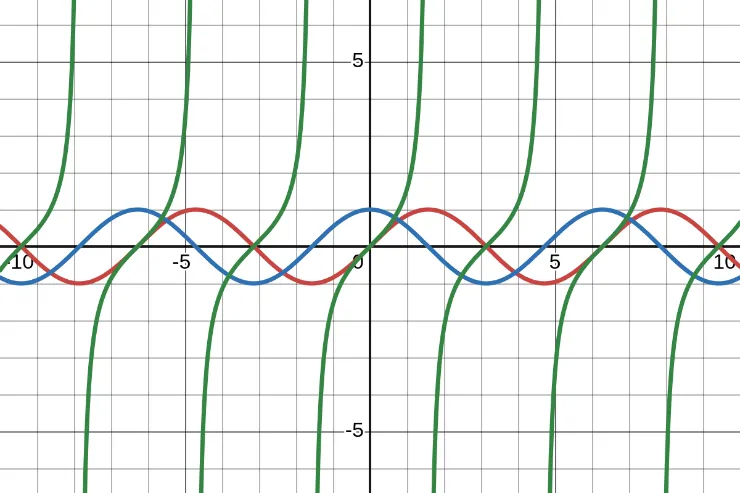
The red line is \(y = sin(x)\).
The blue line is \(y = cos(x)\).
The green line is \(y = tan(x)\).

Midline, Amplitude, and Period

Midline, amplitude, and period describe key features of periodic (wave-like) graphs, like sine or cosine functions: the midline is the horizontal center line; the amplitude is the vertical distance from the midline to a peak or trough, always positive; and the period is the horizontal length of one full cycle, showing where the wave pattern repeats. Here are examples.

from Graph

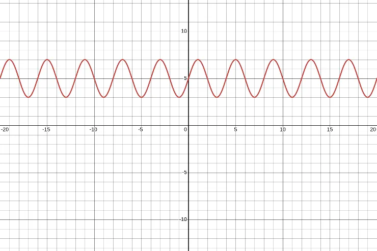
Given the graph of a sinusoidal function, we can analyze it to find the midline, amplitude, and period.

The horizontal line that passes exactly between ‍\(y = 7\)(the maximum value) and ‍\(y = 3\) (the minimum value) is ‍\(y = 5\), so that's the midline.

The vertical distance between the midline and any of the extremum points is ‍2, so that's the amplitude.

The distance between the two consecutive maximum points is ‍4, so that's the period.

from Equation

Determine the amplitude and the period of \(y = \textcolor{yellow}{-\frac{1}{2}}\cos(\textcolor{yellow}{3}x)\).

The amplitude is \(|-\frac{1}{2}| = \frac{1}{2}\).
The period is \(\frac{2\pi}{|3|} = \frac{2\pi}{3}\).

Sinusoidal Models

Let's write trigonometric functions that model these examples.

In Johannesburg in June, the daily low temperature is usually around \(\textcolor{yellow}{3^{\circ}C}\), and the daily high temperature is around \(\textcolor{yellow}{18^{\circ}C}\). The temperature is typically halfway between the daily high and daily low at both 10 AM and 10 PM, and the highest temperatures are in the afternoon.

Temperature \(T\) in Johannesburg \(t\) hours after midnight is \(T(t) = (\frac{18 - 3}{2})\sin(\frac{\pi}{12}(t - 10)) + (\frac{18 - 3}{2}) + 3 = 7.5\sin(\frac{\pi}{12}(t - 10)) + 10.5\).

The sine function is chosen because it naturally crosses the midline, matching the statement “The temperature is typically halfway between the daily high and daily low at both 10 AM and 10 PM.”
The hottest day of the year in Santiago, Chile, on average, is January 7, when the average high temperature is \(\textcolor{yellow}{29^{\circ}C}\). The coolest day of the year has an average high temperature of \(\textcolor{yellow}{14^{\circ}C}\).

How many days after January 7 is the first spring day when the temperature reaches \(20^{\circ}C\)? Remember that January 7 is in the summer in Santiago and, using 365 days as the length of a year.

\(T(d) = \frac{29 - 14}{2} \cos(\frac{2\pi}{365}d) + \frac{29 - 14}{2} + 14 = 7.5 \cos(\frac{2\pi}{365}d) + 21.5\)

Cosine was chosen because January 7 corresponds to a peak, and cosine naturally models a maximum at the starting point — making the equation simpler and more intuitive.

Modelling

Mathematical modeling is the process of using mathematical language, equations, and concepts to represent, analyze, and predict the behavior of real-world systems or problems.

Modelling with Function Combination

Modeling with function combination uses basic operations (add, subtract, multiply, divide) and composition (\(f(g(x))\)) to build more complex mathematical models that better represent real-world situations by merging simpler functions. Here is an example.

Ify is building a tree tower, which is a tower built on the top of a tree! The tree is currently 5 meters tall, and Ify has found it is growing by 0.1m a month. The tower is currently 2m tall, and Ify adds to it about 0.2m a month.

The function \(A(m)\) returns the tree's height (in meters) \(m\) months from now, \(A(m) = 5 + 0.1m\).

The function \(B(m)\) returns the tower's height (in meters) \(m\) months from now, \(B(m) = 2 + 0.2m\).

The function \(C(m)\) returns the vertical distance (in meters) between the ground and the top end of the tower \(m\) months from now, \(C(m) = A(m) + B(m) = 7 + 0.3m\).

Manipulating Formulas

Formula manipulation is rearranging a mathematical equation to solve for a different variable, using inverse operations (add/subtract, multiply/divide) on both sides to keep it balanced, just like solving for numbers, but treating variables as single units.

As an example, we can go back to the Algebra (Part 2), Inverse Functions. There is an example of converting degrees Celsius to Fahrenheit.

Reference

The best way to learn is to practice more. You may notice that this article lacks examples, particularly in the Modelling section. That is because this article is designed to conclude some topics in a single article. To practice more, I recommend that you go to the primary source/reference.

The primary reference is Khan Academy, with assistance from ChatGPT and Gemini as well.